Analysis and visualizations of the palmerpenguins dataset
This analysis used the palmerpenguins dataset to explore how species, body mass, and bill dimensions relate. It offers a concise, reproducible example of data wrangling, visualization, and interpretation for the web.
Research question
What are the morphological differences in bill length, depth, and body mass among penguin species, and how do these traits vary across islands?
Intended audience
This page is aimed at students, educators, and data science enthusiasts learning data exploration and visualization in R.
Data source
I used the palmerpenguins dataset hosted by the palmerpenguins project:
Data (CSV): https://raw.githubusercontent.com/allisonhorst/palmerpenguins/master/inst/extdata/penguins.csv
Data dictionary
The Data dictionary, containing full variable descriptions can be found here: https://rpubs.com/rich_i/dd_pp
Key variables used in this dataset include:
species: species of penguin (Adelie, Chinstrap, Gentoo)
island: island name
bill_length_mm: bill length (mm)
bill_depth_mm: bill depth (mm)
flipper_length_mm: flipper length (mm)
body_mass_g: body mass (g)
sex: sex of the penguin (male/female)
year: the year of study (2007, 2008, and 2009)
ImportantExpand to see data information
This is a quick reminder about the research question and the data source.
Question: morphological differences in species and variance by island.
Data: palmerpenguins CSV (linked above).
Data wrangling and inspection
We load the tidyverse (dplyr, tidyr, ggplot2) to clean and reshape the data using functions like filter, select,mutate, arrange, group_by, summarize, and drop_na.
NoteData and reproducibility
The data is loaded directly from the project’s CSV URL, allowing this page to render reproducibly without relying on the palmerpenguins package.
# load librarieslibrary(readr)library(dplyr)
Attaching package: 'dplyr'
The following objects are masked from 'package:stats':

    filter, lag
The following objects are masked from 'package:base':

    intersect, setdiff, setequal, union
library(tidyr)library(ggplot2)# read data from raw CSVpeng <-read_csv("https://raw.githubusercontent.com/allisonhorst/palmerpenguins/master/inst/extdata/penguins.csv")
Rows: 344 Columns: 8
── Column specification ────────────────────────────────────────────────────────
Delimiter: ","
chr (3): species, island, sex
dbl (5): bill_length_mm, bill_depth_mm, flipper_length_mm, body_mass_g, year

ℹ Use `spec()` to retrieve the full column specification for this data.
ℹ Specify the column types or set `show_col_types = FALSE` to quiet this message.
# Wrangle: keep key variables, drop missing values, create a mass_kg variable, filter to common speciespeng_clean <- peng %>%select(species, island, bill_length_mm, bill_depth_mm, flipper_length_mm, body_mass_g, sex) %>%drop_na(bill_length_mm, bill_depth_mm, body_mass_g, sex) %>%mutate(body_mass_kg = body_mass_g /1000,bill_ratio = bill_length_mm / bill_depth_mm) %>%filter(species %in%c("Adelie", "Chinstrap", "Gentoo")) %>%arrange(species, island)# Quick summary table by speciessummary_by_species <- peng_clean %>%group_by(species) %>%summarize(n =n(),mean_mass_g =mean(body_mass_g),sd_mass_g =sd(body_mass_g),mean_bill_length =mean(bill_length_mm))summary_by_species
Overall, Gentoo penguins tend to be heavier with longer bills than Adelie and Chinstrap species.
Visualizations
Below, three visualizations are then created with different geom_*() functions, complete with titles, subtitles, captions, and readable axis labels. One includes faceting
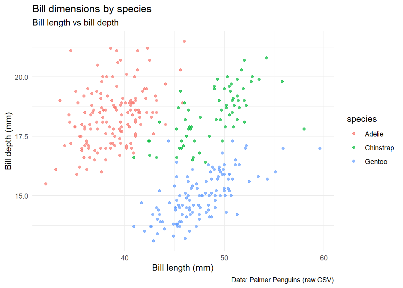
1. Scatter: bill length vs bill depth (geom_point)
ggplot(peng_clean, aes(x = bill_length_mm, y = bill_depth_mm, color = species)) +geom_point(alpha =0.7) +labs(title ="Bill dimensions by species",subtitle ="Bill length vs bill depth",caption ="Data: Palmer Penguins (raw CSV)",x ="Bill length (mm)",y ="Bill depth (mm)") +theme_minimal()
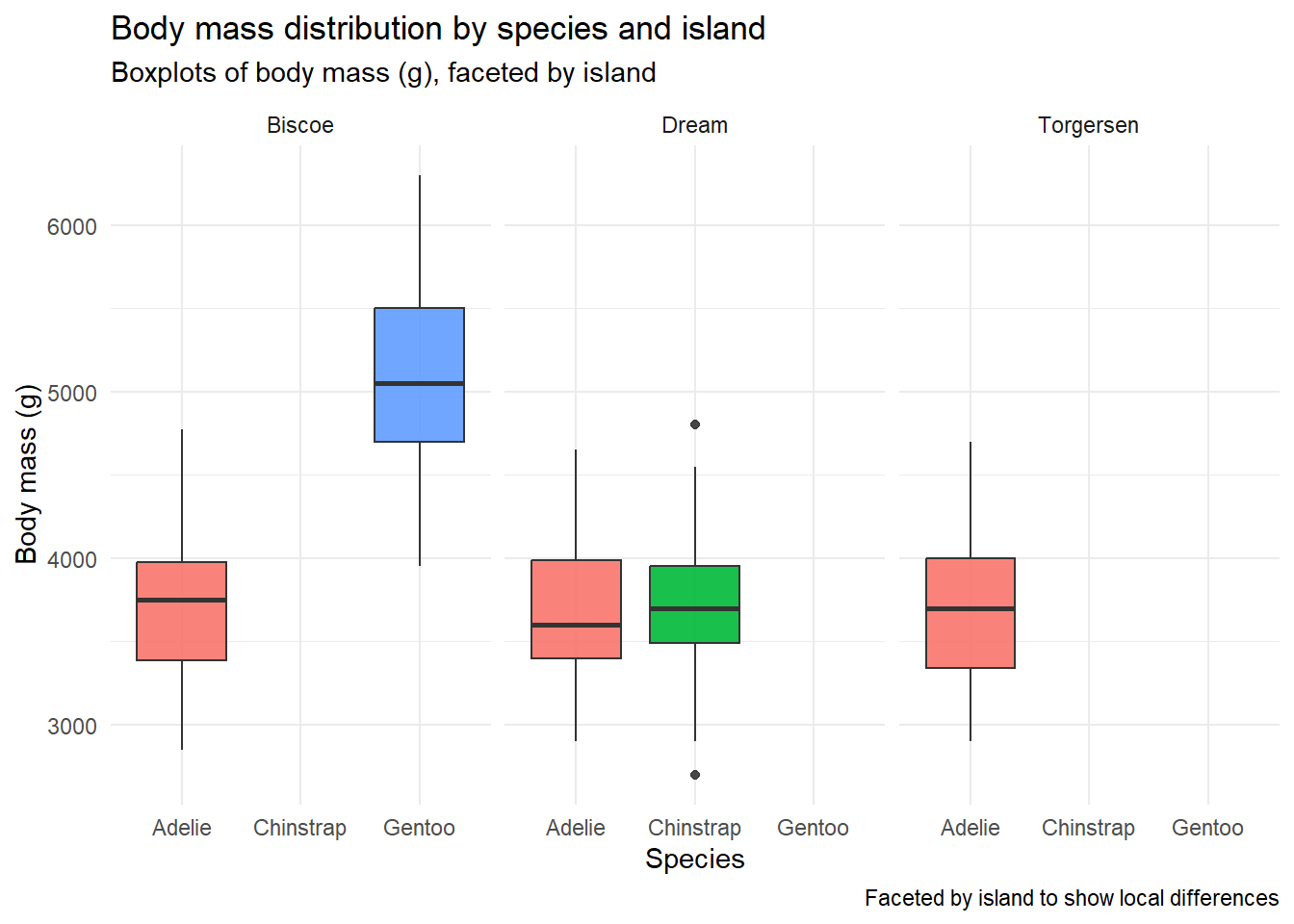
2. Boxplots: body mass by species (geom_boxplot) with faceting by island
ggplot(peng_clean, aes(x = species, y = body_mass_g, fill = species)) +geom_boxplot(alpha =0.9) +facet_wrap(~ island) +labs(title ="Body mass distribution by species and island",subtitle ="Boxplots of body mass (g), faceted by island",caption ="Faceted by island to show local differences",x ="Species",y ="Body mass (g)") +theme_minimal() +theme(legend.position ="none")
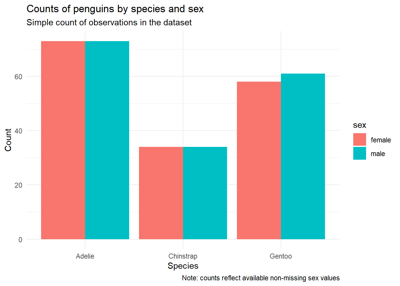
3. Bar chart: counts by species and sex (geom_bar)
ggplot(peng_clean, aes(x = species, fill = sex)) +geom_bar(position ="dodge") +labs(title ="Counts of penguins by species and sex",subtitle ="Simple count of observations in the dataset",caption ="Note: counts reflect available non-missing sex values",x ="Species",y ="Count") +theme_minimal()
This brief analysis shows that Gentoo penguins generally have greater body mass and longer bills than Adelie and Chinstrap species. Faceting by island highlights subtle local differences, suggesting possible ecological influences. The bill length–depth scatterplot reveals partial species separation with some overlap, pointing to the value of multivariate approaches like PCA. Overall, the page illustrates simple, reproducible steps for data wrangling, visualization, and quick exploratory analysis.
References
This page includes citations for the dataset and core software, listed in the bibliography section.